And we can shift the $H(t)$ by $T$ time, that is $H(t-T)$.
The delta function $$\delta (t) is always 0, except for a single time point $t=0$, it has a value 1. Thus delta function is all in one instant, an impulse. Also, the delta function can be shifted by $T$ time, that is $\delta (t-T)$.
Although this is not a continuous function, this is what we do in real life. Because the deposits are always made at some specific instants.
where $s$ is the running clock, and $t$ is the time we look at it. Why the integral term has $(t-s)$ inside? Because the deposits $q(s)$ is made at time point $s$, and you only get interests after you made the deposits.
Here is the part that we get oscillation input, the $\cos\omega t$ part. Or we can think that's a vibration part, or any thing related to circular motion.
$$\frac{dy}{dx}=ay+\cos\omega t$$ when $y=y(0)$ at $t=0$. Look for $y_p(t)=M\cos\omega t+N\sin\omega t$.
This series will be my personal notes on differential equations (including ordinary differential equation (ODE), partial differential equation (PDE) and stochastic differential equation (SDE)). These posts may contain mistakes.
The first a few posts will be different solutions for different forms of first order ODE.
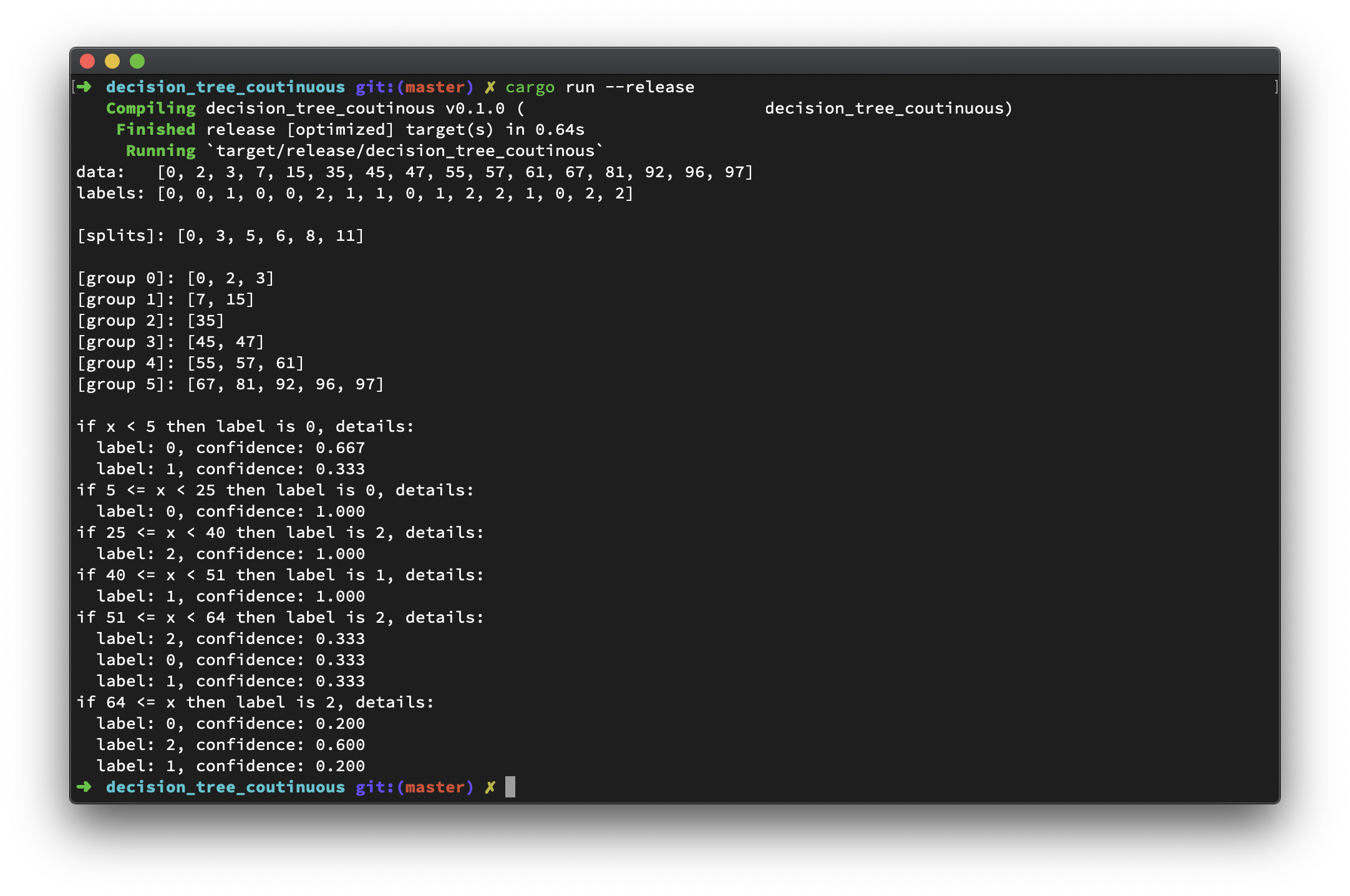
This post has two main purposes, 1) serves as personal notes for handling continuous features in decision tree; 2) try to use trait to add more computation operations to vectors, because the original Vec shipped with Rust is nowhere near the numpy in Python when it comes to scientific computation. (Though I know that Vec may not be designed to do handle such task.)
There are many ways to handle continuous descriptive features, such as discretions. This post will exploit weighted variance as a measurement for splitting continuous feature at a node.
The weighted variance is computed by the following equation, where $n$ is the number of rows in the data, $\mathcal{L}$ is the set of all unique labels, $D$ is the column with continuous features ($n$ rows), $p^*$ denotes the best split position in $D$.
Once the algorithm decides the best split position of $D$, we can apply divide and conquer! For example, if $p^*$ has been computed, then we recursively apply this mechanism to both $D[0 .. p^*]$ and $D[p^* ..]$. When the split position arrays, $S_i$ and $S_j$, of $D[0 .. p^*]$ and $D[p^* ..]$ return, $S_i$ and $S_j$ will be merged and sorted as final value.
For the match Limp Stoners vs Exmouth Breathers the two bookmakers A and C offer different odds,
Stoners Win
Draw
Breathers Win
A
4/1 (5.00)
3/1 (4.00)
2/3 (1.67)
C
3/1 (4.00)
2/1 (3.00)
1/1 (2.00)
You have £100. How do you have to place your bets in order to maximize guaranteed profit no matter what the outcome of the game?
Noticing,
One is allowed to put money on different outcomes simultaneously. So, you can bet £50 on Stoners and £20 on Draw at A, and £30 on Breathers at C.
The numbers for the odds mean that, for example, if you bet £1 on Stoners at BrokeLads you will get £5.00 back (your own £1 and £4 winning). The fraction format specifies how much you would win if you bet £1, the decimal format specifies how much you would get back if you bet £1 (so, it’s the same as the fraction + 1.
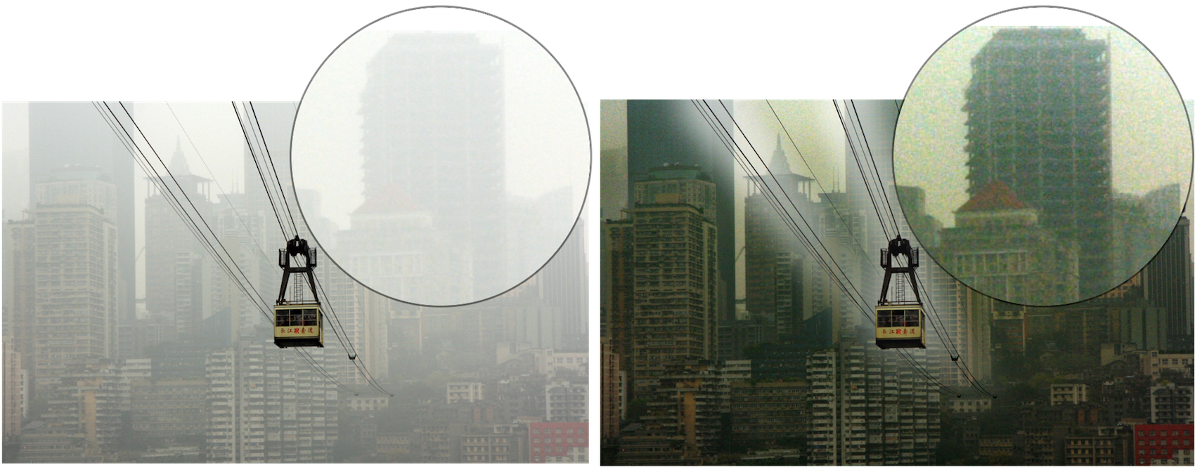
It is based on a key observation most local patches in haze-free outdoor images contain some pixels which have very low intensities in at least one color channel.
Last, the haze removal can produce depth information and benefit many vision algorithms and advanced image editing. Haze or fog can be a useful depth clue for scene understanding. The bad haze image can be put to good use.
我们可以简单的将$\mathbf{x}$理解为图像中的某一个位置,那么,$\mathbf{I}(\mathbf{x})$则是我们最终观察到的有雾的图像在该点的强度;$\mathbf{J}(\mathbf{x})$是在没有雾的情况下,该点应有的强度;$t(\mathbf{x})$是该点的透射率(the medium transmission describing the portion of the light that is not scat- tered and reaches the camera);最后,$\mathbf{A}$是全局大气光强(global atmospheric light)。